Laffer Curve

                                                       

Everybody’s Got A Laughing Place

Everybody's got a laughin' place,
A laughin' place, to go ho-ho!
Take a frown, turn it upside-down
And you'll find yours I know ho-ho!

But nobody needs a Laffer Curve!

The Laffer Curve attempts to explain the revenue from an income tax with the rate of that income tax. It does so by assuming that this curve can be explained by a parabola. IMHO that is why there is a problem. It assumes that the sweet spot, maximum, is where the first derivative of the parabola is zero. IMHO, the curve should NOT be a single parabola but instead should be two intersecting hyperbolas. That is why there is a problem. A parabola requires that for incomes below a zero tax rate, the tax revenue be negative, and the income be imaginary, and at tax rates more than 100% the revenue be negative, and the income be imaginary.  A hyperbola approaches zero revenue, but never becomes zero or negative, and thus the  income never becomes imaginary.

A single parabola can look like two intersecting hyperbolas, but these looks can be deceiving. This behavior is better explained as the lower portion of two intersecting hyperbolas. These hyperbolas are in fact inverses of each other and the point of intersection is also defined. The tax rate should be 16.7% (1/6) of total income. This is the median tax rate, NOT the highest tax rate. If the median is 16.7%, and the lowest effective tax rate is 0%, then the highest tax rate in a normal distribution should be 33.4%. This is the effective rate, not the marginal rate. The effective tax rate is like speed; the marginal tax rate is like acceleration. They are NOT the same and should not be confused with each other. The marginal rate in tax tables depends on the number of equal tax brackets. The marginal tax rate is the percentage of the maximum tax rate which applies.  The effective tax rate is the marginal rate multiplied by that maximum rate. The tax rates should change from the lowest effective rate of 0% to the highest effective tax rate of 33.4% and the lowest income in the highest bracket should be close to the normal  maximum income. If the median household income is $74,580, in 2022 US dollars as reported by the US Census, then the normal maximum income should be twice that, $149,160 in 2023 USD income. According to the U.S. Census Bureau, the mean household income in the United States in 2022 was $105,555. If income was normally distributed, and the median is 50% then the maximum should be twice the median in a normal distribution . To still be normal if skewed, the highest income should not exceed $233,063, 2/ln(2) or ~π Times the Median Income.. The mean income should ideally be half of the highest income. The highest income tax bracket for married filing jointly in the 2023‑24 IRS tax code begins at  $693,750 and there are 7 brackets. The tax brackets using this, as well as the other highest incomes, and the 7 tax brackets are shown in the table below.

The tax brackets are only a linear approximation of what is a non-linear function.  The Census mean income occurs in the 3rd of the 7 brackets in the current IRS tables, but these tables have unequal income brackets. If the income brackets are equalized, but the highest Tax Code income is retained, then the Census mean income occurs in the 2^nd of the 7 brackets . If the highest income is π times the Census median income, then the Census mean income occurs as it should in the 4^th, middle, of the 7 income brackets.

This sounds counter-intuitive, but it is mathematically consistent. Most of the tax revenue comes from the lowest tax brackets. This is because while the rate per taxpayer is low, there are many more taxpayers in these brackets, so that the total revenue from these brackets is very high. The fixation on the rates paid by the few taxpayers in the highest brackets instead of the revenue from the majority of taxpayers in the lowest brackets has been distorting public policy. 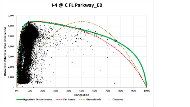By confusing marginal (second derivative) and effective (first derivative) tax rates, by having unequal tax brackets, and by using the Laffer Curve, this is inconsistent with other observations, for example observations of traffic in Florida. Those observations of traffic also suggest that the majority of observations occur before the highest volume. Those observations do NOT support a regular ( such as the one proposed by Greenshields) or irregular (highly sewed such as the one proposed by Van Aerde) parabola, but instead intersecting hyperbolas where the intersection  occurs at 1/6^th of the variance, range of congestion ( similar to tax rates in the Laffer Curve.)

Those who don’t learn from history are doomed to repeat it. Those who don’t know math are doomed to be conned.

References

Greenshields, B. (1935). A study of traffic capacity. Highway Research Record, (pp. 448-477). Washington, DC.

Van Aerde, M. (1995). A single regime speed-flow-density relationship for freeways and arterials. Washington D. C.,: Presented at the 74th TRB Annual Meeting,.

 

 

Kamala Harris II

 

Joshua fit the Battle of Jericho.

Know you've heard about Joshua
He was the son of Nun
He never stopped his work until
Until the work was done

God knows that
Joshua fit the battle of Jericho
Jericho, Jericho
Joshua fit the battle of Jericho
And the walls come tumbling down

Joshua meet Kamala.

Kamala Harris, the modern Joshua to Joe Biden’s Moses, tonight accepts the torch as the Presidential nominee of the Democratic Party.  This November, in addition to a glass ceiling shattering, expect the walls to come tumbling down. MAGA better get the name right.  When she fights, she wins!  Not going back!

Limits

 

Camelot

It's true! It's true! The crown has made it clear
The climate must be perfect all the year
A law was made a distant moon ago here:
July and August cannot be too hot
And there's a legal limit to the snow here
In Camelot

Are God’s limits your limits?

The alliance, and the mistake they make, between no-tax conservatives and social conservatives can be explained by mathematics.  No-tax conservatives are opposed to any group. They are what mathematicians would call User Optimalists.  That means they are opposed to “communists” who are by definition believers in a group. Social conservatives are not opposed to a group, a system, after all they believe in God who is a group, as long as that group agrees with them.  They are what mathematicians would call System Optimalists. They are opposed to Communists because Communists are atheists, and they are not. After all the father of modern Communism, Karl Marx, said that religion is the opiate of the people. In fairness, Robespierre and the other French Revolutionaries were anticlerical because, historically, organized religion has supported the ruling class, so Karl Marx was by no means the first to confuse anti-clericalism with atheism.

It is possible to believe in a group and thus support taxes for the group,  and still believe in God.  This all stems from the belief that God is everywhere, therefore where God is not must be zero. And also that God is without, has zero, error. A mathematician would state both of these as 0±0.  This is decidedly NOT the mean, µ, of the group has no error, ε, which a mathematician would state as µ±ε. While 0±0 is true if either µ=0 or ε=0, it is not limited to only these values.  God’s mean, µ, is zero BECAUSE 0=µ-µ.  God’s error is zero because limit n→∞  ε=σ/√n =0, NOT because God’s Standard Deviation, σ, is zero. 

The problem is that  the square of a Standard Deviation, σ², for example God's of π²/36, can be observed even if God can not.  For example in my field of traffic engineering, σ² might be the observable Free Flow Speed.  At the same time traffic engineers can observe the capacity of a road, but the arrival volume of the road can exceed the capacity of the road and can NOT be observed. This only requires that the mean is NOT half of the observable capacity, it only acknowledges that the arrival volume can not be observed.  The mean, which is half of the total value of sample, can exceed what can be observed.  But if you can’t observe the mean, that does not mean that the mean must be zero. 

No-tax conservatives observe and concede that σ²≠0 but insist that the mean must be zero.  Social conservatives concede that the mean is not zero, but that σ=0.  No-tax conservatives believe that they are privileged, not lucky,  that there is no value in being unlucky and that there is no value in helping anyone who is unlucky, where luck is defined by both µ and σ.  Social conservatives, will help the unlucky in their own group and believe that the only groups that should be helped are those who believe like them, have a σ=0, the difference between the other group and their group.  The alliance between these positions requires social conservatives to support behavior that is µ=0 even if they believe it is not, and no-tax conservatives to support behavior that is σ=0, even if they know that it is not.

The fact that Republicans have this alliance goes back to its beginnings in the 1850s, when no-tax Whigs who were anti-slavery and anti-immigrant Know-Nothings who were anti-slavery were welcomed into the Republican party.  Dixiecrats, who were pro-slavery and  eventually pro-Jim Crow, were part of the Democratic Party until LBJ, and Nixon’s Southern Strategy. Anti-slavery was eventually replaced by the abortion issue, which no-tax conservatives have no intention of supporting but will support social conservatives who do support it.  And that is why single-issue politics are so dangerous. They lead to dangerous alliances. Democrats observe that there is a group, and act like its mean is God’s mean even if God’s mean is unobservable. But once upon a time the fiscally conservative but social liberals, e.g Mark Twain who was a Mugwump Republican or Nelson Rockefeller who was responsible for the eponymous last name attributed to Everett Dirksen, Howard Baker, Gerald Ford and others as Rockefeller Republicans, believe that there is a group, and act like its mean is God’s mean even if God’s mean is unobservable.  They would be like Adam Kinzinger, George Conway or Rick Wilson and drummed out of the current Republican Party as RINOs .  They act like moderate Democrats in believing that u≠0 and σ≠0 is consistent with 0±0 for God.  Being a communist only means that you don’t believe in a ruling class, not that you don’t believe in God. The Evangelical Protestants have rejoiced in the Supreme Court overturning Roe v. Wade even though they do not agree with most other things with the mostly Roman Catholic Supreme Court justices who actually overturned this case.

To be very nerdy, the best strategy is a Nash Equilibrium which mathematically is to act like your group variance is 5/6 * σ²  AND µ>0.  Moderate Democrats and Moderate Republicans unite! You may not know what the unobservable is, but you know it exists and you know your limits.

Shapes

 

Aquarius/Let the Sunshine In

Harmony and understanding
Sympathy and trust abounding
No more falsehoods or derisions
Golden living dreams of visions
Mystic crystal revelation
And the mind's true liberation
Aquarius
Aquarius

The “Age of Aquarius” is also the “Age of 'The Twilight Zone'”

“There is a fifth dimension beyond that which is known to man. It is a dimension as vast as space and as timeless as infinity. It is the middle ground between light and shadow, between science and superstition, and it lies between the pit of man's fears and the summit of his knowledge. This is the dimension of imagination. It is an area which we call ‘The Twilight Zone’”

Viewers of the old TV series, or visitors to Walt Disney World’s “Twilight Zone” Tower of Terror might recognize this intro. Have you ever thought about what this means? The first three dimensions are the dimensions of space: length, width, and height. The fourth dimension is that of time. Minkowski developed a transform to combine the three dimensions of space into a 2-D chart of space‑time, which his student Einstein would later make much more famous. Mathematicians would call the fifth dimension i, the imaginary number which is the square root  of minus 1, √-1,   If you rotate the surface of space-time around the axis of imagination you will develop a three-dimensional volume of the “Twilight Zone”.  So what should the surface be?

A function, as opposed to an equation, is one which has only one solution for each input value. There are four families of functions:

·       Linear, f(x) = y = a *x +b;

·       Power, f(x) = y = a * xⁿ +b;

·       Exponential, f(x) = y = a* e^b*x; and

·       Logarithmic, f(x) = y = a + b * ln(x)

The logarithmic function is the inverse, f^-1(x), of an exponential function, therefore it is convenient to combine these into one surface, hyperbolic, which means that there are three surfaces. Some other hyperbolic functions are the hyperbolic sine, hyperbolic cosine, hyperbolic tangent, etc., and all of these can be expressed as exponentials. Similarly the regular circular trigonometric functions: sine, cosine, tangent, etc., can all be expressed as series of power functions, and it is conventional to call their surface spherical. Because it is NOT possible to express linear functions as either hyperbolic or circular trigonometric functions, and both spherical and hyperbolic surfaces are also curved, it is convenient to call a linear surface flat. It is also conventional to call flat surfaces Euclidean and both spherical and hyperbolic surfaces non-Euclidean.

 The surfaces, their functions, inverses, domains, and ranges are:

	Function	Domain	Range		Inverse	Domain	Range
Flat	a*x+b	-∞ to ∞	-∞ to ∞		(x-b)/a	-∞ to ∞	-∞ to ∞
Spherical	a*xn +b	-∞ to ∞	-∞ to ∞		n√((x-b)/a)	-∞ to ∞	-∞ to ∞	(x-b)/a >0 or else imaginary solution  when n is even
Hyperbolic	a*eb*x	-∞ to ∞	a* to ∞	if a is  positive	ln(x/a)/b	-∞ to ∞	0 to ∞	ln(x) is not defined for negative numbers
			-∞ to a*	if a is negative

* The starting point of the range varies with the hyperbolic function. For example  cosh(x) has a range of 1 to ∞, but cosh(x)=½(e^x+e^-x) which requires that for it a is 1.

As shown in the table above, a real number as an input to the inverse function becomes an imaginary number as an output on a spherical surface. A real input added to a zero imaginary number is indistinguishable from a complex number whose coefficient of the imaginary component is zero. It is suggested that the input should allow real or complex numbers without the inverse requiring a change in the case of number for its output solution. Additionally spherical surfaces are finite in reality, which is a consequence of the circular identity, cos²+sin²=1. Circular trigonometric functions are infinite and repeating, but they repeat with a period of 2π. Hyperbolic surfaces have two domains, and those domains can accommodate either real or complex numbers as inputs. This is because of the hyperbolic identity cosh²‑sinh²=1 and the fact the hyperbolic trigonometric functions are infinite and repeating, but only in imaginary surfaces, planes. That is they have a period of 2πi.

The universe appears to be infinite, which rules out its surface being spherical. It must be either flat or hyperbolic. But if the surface is flat then the variance, σ², of that surface must be zero and if there is any transition  between domains it must be at ½, 50%, of σ. However observations of traffic, fluid, etc. suggest that there is a transition, but it occurs not at 50% of σ, but closer to 85% of σ. This is consistent with design recommendations for a road at the 100th highest volume, the dividing line between Level Of Service, LOS, C and D of traffic, the parametric rail capacity of 85%, a speed limit being set at the 85^th percentile of a speed study, etc. The transition point, if the surface is hyperbolic, would be 5/6 σ² or 83.3% of σ. It is noted that the Nash Equilibrium is also at 5/6 σ².

If the surface is hyperbolic and the input is complex with a coefficient of zero for the imaginary axis, then σ=1.0579, which is not appreciably different than the solution on a flat surface of σ=1. Since the absolute is by definition twice its mean/median, this means that the absolute on a hyperbolic surface is a random number because that absolute has a mean/median and a variance.

This is not appreciably different than acknowledging that the distances on the surface of the Earth are round by saying ”Distances are locally flat, but globally spherical.” The corresponding statement for space would be “Space is locally flat, but universally hyperbolic.”  This does mean that Pythagoras’ Theorem is c=ln(cosh(a²+b²)), not
c=√(a²+b²) and that the relativistic dilation factor is γ=ln(cosh(1-v²/c²), not γ=√(1‑v²/c²). Melkhout( (Mabkhout, 2012) did propose that the universe has a hyperbolic shape and that by assuming this and solving its Einstein Field Tensors in hyperbolic space the need for Dark Matter and Dark Energy vanishes. Mahout also points out that a hyperbolic shape explains the rotation of galaxies, is consistent with both the age and size of the universe at large scales and  Planck Energy and Planck length at small scales, and a hyperbolic shape that is almost flat is consistent with a period of initial but short inflation after the Big Bang. It is proposed that not only is the shape of universe hyperbolic, but the universe is one sheet of a two-sheeted hyperboloid. The Big Bang is the point of intersection between these two sheets.

As to the song lyrics, remember that while the song was from the musical Hair, it was a big recording hit for the singing group the “Fifth Dimension.”

Mabkhout, S. (2012). The infinite distance horizon and the hyperbolic inflation in the hyperbolic universe. Phys. Essays, 25(1), p.112.

 

 

 

Election 2024

The Power of Love

You don't need money, don't take fame
Don't need no credit card to ride this train
It's strong and it's sudden, and it's cruel sometimes
But it might just save your life
That's the power of love
That's the power of love

Not Going Back, except Back to the Future!

The 2024 federal  election is about Making America Great Again, MAGA, versus Not Going Back. In other words the election is about the past versus the future. As such it is fitting that the candidate for MAGA is Donald Trump, whose character served as the model for the villain Biff Tannen in the movie, Back to the Future.  https://www.imdb.com/news/ni59124081/

The American electorate is like George McFly who finally stood up to the bully Biff, which allows Marty to go Back to the Future. https://youtu.be/So2yJzFOJeo?si=-UIbEpI1Q2fT9Dkg. Kamala and Tim, that is where America wants to go too!

Honor Joe Biden!

 

Chad Gayda

Then came the Holy One, blest be He,
And destroyed the angel of death
That slew the butcher
That killed the ox
That drank the water
That quenched the fire
That burned the stick
That beat the dog
That bit the cat
That ate the kid my father bought for two zuzim.
Chad Gadya, Chad Gadya

Chad Gadya Joe Biden!

How should next Monday’s Democratic national convention honor Joe Biden? Will he be remembered in the future? The song above is song by children after a Passover seder.  Every Passover Moses is remembered, even though it has been more than thousands of years. Moses was an adopted Prince of Egypt, who gave it all up to lead the People of Israel in service to the Holy One. Not only did Moses free the Israelites from slavery in Egypt, part the Red Sea, receive the Ten Commandments, and lead the Israelites in the desert, but he did not enter the Promised Land.

“Then Moses went out and spoke these words to all Israel:  “I am now a hundred and twenty years old and I am no longer able to lead you. The Lord has said to me, ‘You shall not cross the Jordan.’ The Lord your God himself will cross over ahead of you. He will destroy these nations before you, and you will take possession of their land. Joshua also will cross over ahead of you, as the Lord said.” Deuteronomy 31:1-4.

Sound familiar? Will you be fondly remembered, Joe Biden? Oh you WILL be fondly remembered, ....you definitely WILL be fondly remembered..... if not for thousands of years, for a very long time.  Joe, come on in and sit a spell. There will always be a place at the table for you!

Tim Walz

 

I am the Walrus

I am the eggman,
They are the eggmen,
I am the walrus,
Goo goo g' joob.

I might be the walrus, but Tim Walz is a batman!

Not THE Batman, the Dark Knight. Alfred is Batman’s batman, just as Sancho Panza is Don Quixote’s batman, Bernardo is Zorro’s batman, Bunter is Lord Peter Wimsey’s batman and Samwise Gamgee is Frodo Baggins’s batman.  Batman comes from the French word for pack.   It is a term for the orderly, typically a common enlisted man, who served, carried the pack, for a British officer.  That officer might be able to do great things for the group, but only with the assistance of his batman.  That batman might sometimes disagree with that officer but kept his promise to serve that officer as long as that officer served the group. I'm with Master Sergeant Walz, how about you?